The one-dimensional minimization subproblem of Stochastic Dual Coordinate Ascent (SDCA) Algorithm
A few years ago, Martin Takáč asked his students (I was one of them) to implement Stochastic Dual Coordinate Ascent SDCA algorithm as part of his ISE 407 final project. After implementing SGD, I didn’t have any time for SDCA. So I didn’t finish it at that time. I have a yearning to finish it as it is a fascinating algorithm. I will be implementing the full SDCA algorithm in the next post but this post is just to derive the one-dimensional minimization problem that arises in the SDCA algorithm. Martin was kind enough to give us the 1D problem directly but we will derive and graph the 1D minimization problem. I will not be discussing the algorithm per se. It is a famous algorithm and the interested reader can get hold of the original paper by Shalev-Shwartz and Zhang (2013). I will merely reproduce a modified version of the algorithm’s pseudocode that Martin gives in his class (they are essentially the same)
Let us take a look at the following steps of SDCA algorithm at an epoch $t$ (as usual we choose the first guess as an all zero vector). My usual caveats exist. The pseudocode is probably correct but I use a different notation than the usual machine learning notation and hence I might have made a few mistakes in some indices. My notation is like this: $m$ = number of observations and $n$ = number of features, $a$ = an observation, $y$ = label, $x$ = current value of the solution and I know that this is bad :(
Step 0: Input: $\alpha^{t}$
Step 1: $\alpha \leftarrow \alpha^{t}$
Step2: Set $w \leftarrow \frac{1}{\lambda m}\sum_{i=1}^{m}a_{i}\alpha_{i}$
Step 1: for iter = 1, … , m, do the following: (Remember, there are m samples):
Step 1a: choose $i \in {1, \dots m} $ randomly
Step 1b: compute $\delta_{i}$ as explained below
Step 1c: $\alpha_{i} \leftarrow \alpha_{i} + \delta_{i}$ (we just update one element of vector $\alpha$)
Step 1d: $x \leftarrow x +\frac{1}{\lambda m}a_{i}$
Step 2: $\alpha^{t+1} \gets \alpha$
Step 3: $x$ can be used to calculate the training error, duality gap etc.
Let us talk more about Step 1b: Without going deep into duality explanation, assuming that we are using logistic loss function, The primal problem looks like this (you can find more about this in my previous blog post on Gradient Descent
\[\min_{x \in \mathbb{R}^{n}} P(x) = \frac{1}{m}\sum_{i=1}^{m}L(x;a_i,y_i)) + \frac{\lambda}{2}||x||^2\]Where,
\[L(x; a,y) = \log(1+\exp(-yx^{T}a))\]We can further simplify the above definition of $L(x;a,y)$ as
\[L(u) = \log(1+\exp(-yu)), \text{where } u = x^{T}a\]The Dual looks like this:
\[\max_{\alpha\in\mathbb{R}^{m}}D(\alpha), \text{where}\ D(\alpha) = \frac{1}{m}\sum_{i=1}^{m}-L^{*}_{i}(-\alpha_{i})-\frac{\lambda}{2}\Bigg\lvert\Bigg\lvert\frac{1}{\lambda m}\sum_{i=1}^{m}\alpha_{i}x_{i}\Bigg\rvert\Bigg\rvert^{2}\]We would like to maximize the above problem to get the solution. The most important thing you have to notice in the dual is the $L^{*}$ which is the conjugate function of $L$. Step 1b asks us to solve
\[\max_{\delta_{i}}\ -L_{i}^{*}(-(\alpha_{i}+\delta_{i})) -\frac{\lambda m}{2}\Big\lvert\Big\lvert x + \frac{1}{\lambda m}a_{i}\delta_{i}\Big\rvert\Big\rvert^{2}\]Though Shalev-Scwartz and Zhang provide it as a maximization problem I prefer it to be a minimization problem like this:
\[\min_{\delta_{i}}\ L_{i}^{*}(-(\alpha_{i}+\delta_{i})) +\frac{\lambda m}{2}\Big\lvert\Big\lvert x + \frac{1}{\lambda m}a_{i}\delta_{i}\Big\rvert\Big\rvert^{2}\]I personally think it looks nice as a minimization problem. Anyway, We have to calculate $L_{i}^{*}(-(\alpha_{i}+\delta_{i}))$ now.
In General, the conjugate of a $f(a)$ is given by
\[f^{*}(b) = \sup_{a}\ b.a - f(a)\]Interested reader can read more about convex conjugate on wikipedia but let us derive the value of $L_{i}^{*}(\alpha)$. To ease some confusion with same symbols appearing again and again, We use the function variable as $u$ and conjugate function variable as $b$
\[L_{i}(u) = \log(1+e^{-y_{i}u})\]Now, the conjugate of the above function is,
\[L_{i}^{*}(b) = \max_{u} \{b.u - \log(1+e^{-y_{i}u}\}\]From calculus, we can say that maximum occurs at that $u$ when the value of the gradient of $L_{i}^{*}(u)$ is 0.
i.e
\[\frac{d}{du}\Big(b.u - \log(1+e^{-y_{i}u})\Big) = b + \frac{1}{1+e^{-y_{i}u}}.-y_{i}.e^{-y_{i}u} = 0\\\] \[b - \frac{y_{i}}{1+e^{y_{i}u}} = 0\]Solving for u, we get
\[u = \frac{1}{y_{i}}\log(-\frac{y_{i}+b}{b})\]Substituting this value of $u$ in $L_{i}^{*}(b)$, we get (I am showing way too many steps of calculation to you as I had already done it in my workbook)
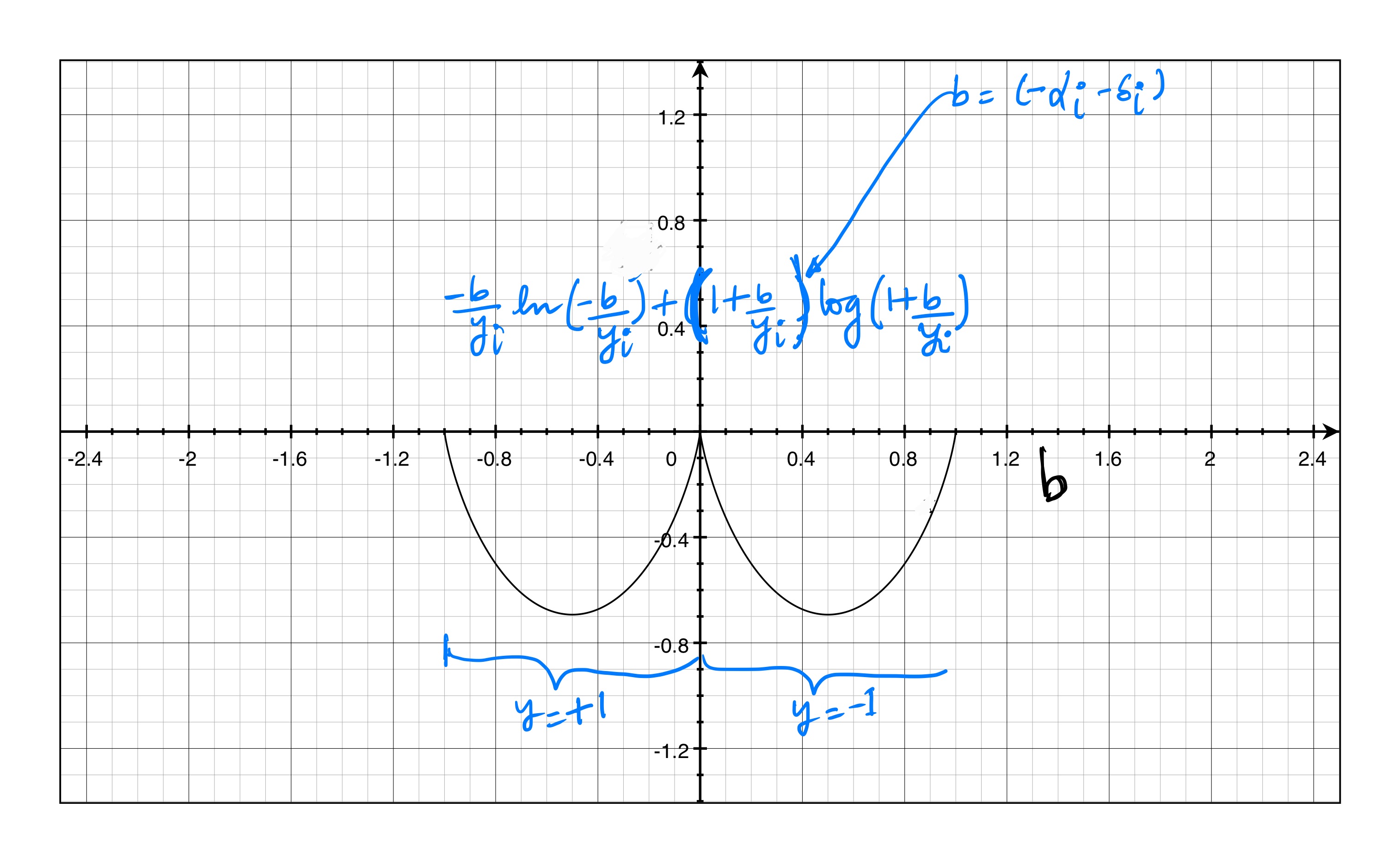
\[\begin{align*} L_{i}^{*}(b) &= \frac{b}{y_{i}}\log(-\frac{b+y_{i}}{b}) -\log(1+e^{-\log(-\frac{b+y_{i}}{b})}) \\\\ &\implies \frac{b}{y_{i}}\bigg[\log(b+y_{i})-\log(-b)\bigg]-\log(1-\frac{b}{b+y_{i}}) \\\\ &\implies \frac{b}{y_{i}}\bigg[\log(b+y_{i})-\log(-b)\bigg]-\log(\frac{y_{i}}{b+y_{i}}) \\\\ &\implies \frac{b}{y_{i}}\log(b+y_{i})-\frac{b}{y_{i}}\log(-b)-\log(y_{i})+\log(b+y_{i}) \\\\ &\implies(1+\frac{b}{y_{i}})\log(b+y_{i})-\frac{b}{y_{i}}\log(-b)-\log(y_{i}) \\\\ &\implies (1+\frac{b}{y_{i}})\bigg[\log(y_{i}(1+\frac{b}{y_{i}}))\bigg] -\frac{b}{y_{i}}\log(-b) -\log(y_{i}) \\\\ &\implies (1+\frac{b}{y_{i}})\log(y_{i}) + (1+\frac{b}{y_{i}})\log(1+\frac{b}{y_{i}}) -\frac{b}{y_{i}}\log(-b) -\log(y_{i}) \\\\ &\implies \frac{b}{y_{i}}\log(y_{i}) -\frac{b}{y_{i}}\log(-b) + (1+\frac{b}{y_{i}})\log(1+\frac{b}{y_{i}}) \\\\ &\implies -\frac{b}{y_{i}}\log(-\frac{b}{y_{i}}) + (1+\frac{b}{y_{i}})\log(1+\frac{b}{y_{i}}) \end{align*}\]So we finally get the above conjugate function.
But this is just a part of the complete 1D minimization problem. The full problem looks like this:
\(-\frac{b}{y_{i}}\log(-\frac{b}{y_{i}}) + (1+\frac{b}{y_{i}})\log(1+\frac{b}{y_{i}}) +\frac{\lambda m}{2}\Big\lvert\Big\lvert x + \frac{1}{\lambda m}a_{i}\delta_{i}\Big\rvert\Big\rvert^{2}\) where $b = (-\alpha_{i}-\delta_{i})$
Remember that this is a 1-D optimizations problem in $\delta_{i}$. Let us plot the conjugate part of the problem. We can see that the plot depends on the value of $y_{i}$ and $y_{i}$ can only be either -1 or +1.
Shout out to Benedikt Bienhüls for his suggestions.